Solving the Travelling Salesman Problem with MiniSom

Have you ever heard of the Travelling Salesman Problem? I'm pretty sure you do, but let's refresh our mind looking at its formulation: "Given a list of points and the distances between each pair of points, what is the shortest possible path that visits each point and returns to the starting point?".
What makes this problem so famous and so studied is the fact that it has no "quick" solution as the complexity of calculating the best path increases adding more points. And the complexity increases so fast that, even with modern hardware, it can be impossible to compute an exact solution in a reasonable time. In more rigorous terms, it is an NP-hard problem. Many heuristics are known to solve this problem and in this post we will see a solution based on Self-organizing Maps (SOM). A SOM is a Neural Network that is capable of mapping an input point into a bi-dimnsional space placing points that are close to each other into the same area. Hence, the idea to solve our problem is to train the SOM in order to map the points to visit in single dimension map and visit the points from the one mapped to the first cell (the one on the left) to the last cell (on the right). Points that are mapped to the same cell are visited consecutively.

Let's generate a set of points to test this idea:

import numpy as np
import matplotlib.pyplot as plt

np.random.RandomState(10)
N_points = 20
N_neurons = N_points*2
t = np.linspace(0, np.pi*2, N_points)
x = np.cos(t)+(np.random.rand(N_points)-.5)*.3
y = np.sin(t)*.8+(np.random.rand(N_points)-.5)*.2
points = np.array([x,y]).T
plt.scatter(x, y)

We can now import MiniSom, our favorite implementation of the Self_Organizing Maps, and see what path it's able to produce:

from minisom import MiniSom

som = MiniSom(1, N_neurons*2, 2, sigma=10,
              neighborhood_function='gaussian', random_seed=50)
max_iter = 2000
som.pca_weights_init(points)

paths_x = []
paths_y = []
for i in np.arange(max_iter):
    i_point = i % len(points)
    som.update(points[i_point], som.winner(points[i_point]), i, max_iter)
    visit_order = np.argsort([som.winner(p)[1] for p in points])
    visit_order = np.concatenate((visit_order, [visit_order[0]]))
    paths_x.append(points[visit_order][:,0])
    paths_y.append(points[visit_order][:,1])
    
plt.scatter(x, y, label='point to visit')
plt.plot(paths_x[-1], paths_y[-1],
         'C3', linewidth=2, label='path')

In the snippet above we initialized the SOM and run 2000 training iterations (check this out to discover how that works). At each iteration we have saved the path found and visualized the last solution. As we can see, the line covers all the points and it's easy to see that it's the best possible path with just a glance. However, it's interesting to see how the solution evolves at each iteration:

from matplotlib.animation import FuncAnimation
from IPython.display import HTML

fig, ax = plt.subplots()
plt.scatter(x, y, label='point to visit')
ln, = plt.plot([], [], 'C3', linewidth=2, label='path')
plt.legend()

def update(frame):
    ln.set_data(paths_x[frame], paths_y[frame])
    plt.title('iteration = %d' % frame)
    return ln,

ani = FuncAnimation(fig, update, frames=np.arange(max_iter),
                    interval=10, repeat=False, blit=False)
HTML(ani.to_html5_video())

Here we note that the initial path is very messy and presents various loops and that the more the network is trained the more optimal the solution becomes. Notice that the snippet above uses the object HTML from the IPython library and it will automatically display the video if a Jupyter notebook is used. The video can be saved in a specific location using ani.save(filename.mp4).

Neural Networks Regularization made easy with sklearn and matplotlib

Using regularization has many benefits, the most common are reduction of overfitting and solving multicollinearity issues. All of this is covered very well in literature, especially in (Hastie et all). Howerver, wihout touching too many details we can have a very straigthforward interpretation of regularization. Regularization is a way to constrain a model in order to learn less from the data. In this post we will experimentally show what are the effects of regularization on a Neural Network (Multilayer Perceptron) validating this interpretation.

Let's define a goal for our Neural Network. We have a dataset H and we want to build a model able to reconstruct the same data. More formally, we want to build a function f that takes in input H and returns the same values or an approximation close as possible to H. We can say that we want f to minimize the following error

To begin our experiment we build a data matrix H that contains the coordinate of a stylized star:

import numpy as np
import matplotlib.pyplot as plt
%matplotlib inline

x= [np.cos(np.pi/2), 2/5*np.cos(np.pi/2+np.pi/5), np.cos(np.pi/2+2*np.pi/5), 
    2/5*np.cos(np.pi/2+3*np.pi/5), np.cos(np.pi/2+4*np.pi/5), 
    2/5*np.cos(3*np.pi/2), np.cos(np.pi/2+6*np.pi/5), 
    2/5*np.cos(np.pi/2+7*np.pi/5), np.cos(np.pi/2+8*np.pi/5),
    2/5*np.cos(np.pi/2+9*np.pi/5), np.cos(np.pi/2)]

y=[np.sin(np.pi/2), 2/5*np.sin(np.pi/2+np.pi/5), np.sin(np.pi/2+2*np.pi/5),
   2/5*np.sin(np.pi/2+3*np.pi/5), np.sin(np.pi/2+4*np.pi/5),
   2/5*np.sin(3*np.pi/2), np.sin(np.pi/2+6*np.pi/5),
   2/5*np.sin(np.pi/2+7*np.pi/5), np.sin(np.pi/2+8*np.pi/5),
   2/5*np.sin(np.pi/2+9*np.pi/5), np.sin(np.pi/2)]

xp = np.linspace(0, 1, len(x))
np.interp(2.5, xp, x)
x = np.log(np.interp(np.linspace(0, 1, len(x)*10), xp, x)+1)

yp = np.linspace(0, 1, len(y))
np.interp(2.5, yp, y)
y = np.interp(np.linspace(0, 1, len(y)*10), yp, y)
#y[::2] += .1

H = np.array([x, y]).T
plt.plot(H[:,0], H[:,1], '-o')

Now the matrix H contains the x coordinates of our star in the first column and the y coordinates in the second. With the help of sklearn, we can now train a Neural Network and plot the result:

from sklearn.neural_network import MLPRegressor
from sklearn.preprocessing import minmax_scale

H = scale(H)

plt.figure()
f = MLPRegressor(hidden_layer_sizes=(200, 200, 200), alpha=0)
f.fit(H, H)
result = f.predict(H)
plt.plot(result[:,0], result[:,1], 'C3', linewidth=3, label='Neural Network')
plt.plot(H[:,0], H[:,1], 'o', alpha=.3, label='original')
plt.legend()
#plt.xlim([-0.1, 1.1])
#plt.ylim([-0.1, 1.1])
plt.show()

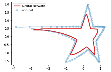
In the snippet above we created a Neural Network with 3 layers of 200 neurons. Then, we trained the model using H as both input and output data. In the chart we compare the original data with the estimation. It's easy to see that there are small differences between the two stars but they are very close.
Here's important to notice that we initialized MLPRegressor using alpha=0. This parameter controls the regularization of the model and the higher its value, the more regularization we apply. To understand how alpha affects the learning of the model we need to add a term to the computation of the error that was just introduced:

where W is a matrix of all the weights in the network. The error not only takes in account the difference between the ouput of the function and the data, but also the size of weights of the connections of the network. Hence, the higher alpha, the less the model is free to learn. If we set alpha to 20 in our experiment we have the following result:

We still achie an approximation of the star but the output of our model is smaller than before and the edges of the star are smoother.
Increasing alpha gradually is a good way to understand the effects of regularization:

from matplotlib.animation import FuncAnimation
from IPython.display import HTML

fig, ax = plt.subplots()
ln, = plt.plot([], [], 'C3', linewidth=3, label='Neural Network')
plt.plot(H[:,0], H[:,1], 'o', alpha=.3, label='original')
plt.legend()

def update(frame):
    f = MLPRegressor(hidden_layer_sizes=(200, 200, 200), alpha=frame)
    f.fit(H, H)
    result = f.predict(H)
    ln.set_data(result[:,0], result[:,1])
    plt.title('alpha = %.2f' % frame)
    return ln,

ani = FuncAnimation(fig, update, frames=np.linspace(0, 40, 100), blit=True)
HTML(ani.to_html5_video())

Here we vary alpha from 0 to 40 and plot the result for each value. We notice here that not only the star gets smaller and smoother as alpha increases but also that the network tends to preserve long lines as much as possible getting away from the edges which account less on error function. Finally we see that the result degenerates into a point when alpha is too high.

Organizing movie covers with Neural Networks

In this post we will see how to organize a set of movie covers by similarity on a 2D grid using a particular type of Neural Network called Self Organizing Map (SOM). First, let's load the movie covers of the top 100 movies according to IMDB (the files can be downloaded here) and convert the images in samples that we can use to feed the Neural Network:

import numpy as np
import imageio
from glob import glob
from sklearn.preprocessing import StandardScaler

# covers of the top 100 movies on www.imdb.com/chart/top 
# (the 13th of August 2019)
# images downloaded from www.themoviedb.org
data = []
all_covers = glob('movie_covers/*.jpg')
for cover_jpg in all_covers:
    cover = imageio.imread(cover_jpg)
    data.append(cover.reshape(np.prod(cover.shape)))
    
original_shape = imageio.imread(all_covers[0]).shape

scaler = StandardScaler()
data = scaler.fit_transform(data)

In the snippet above we load every image and for each of them we stack the color values of each pixel in a one dimensional vector. After loading all the images a standard scaling is applied to have all the values with mean 0 and standard deviation equal to 1. This scaling strategies often turns out to be quite successful when working with SOMs. Now we can train our model:

from minisom import MiniSom

w = 10
h = 10
som = MiniSom(h, w, len(data[0]), learning_rate=0.5,
              sigma=3, neighborhood_function='triangle')

som.train_random(data, 2500, verbose=True)
win_map = som.win_map(data)

Here we use Minisom, a lean implementation of the SOM, to implement a 10-by-10 map of neurons. Each movie cover is mapped in a neuron and we can display the results as follows:

import matplotlib.pyplot as plt
from mpl_toolkits.axes_grid1 import ImageGrid

fig = plt.figure(figsize=(30, 20))
grid = ImageGrid(fig, 111,
                 nrows_ncols=(h, w), axes_pad=0)

def place_image(i, img):
    img = (scaler.inverse_transform(img)).astype(int)
    grid[i].imshow(img.reshape(original_shape))
    grid[i].axis('off')

to_fill = []
collided = []

for i in range(w*h):
    position = np.unravel_index(i, (h, w))
    if position in win_map:
        img = win_map[position][0]
        collided += win_map[position][1:]
        place_image(i, img)
    else:
        to_fill.append(i)

collided = collided[::-1]
for i in to_fill:
    position = np.unravel_index(i, (h, w))
    img = collided.pop()
    place_image(i, img)

plt.show()

Since some images can be mapped in the same neuron, we first draw all the covers picking only one per neuron, then we fill the empty spaces of the map with covers that have been mapped in nearby neurons but have not been plotted yet.

This is the result:

Where to go next:

• Read more about how Self Organizing Maps work here.
• Check out how to install Minisom here.

Solving the Two Spirals problem with Keras

In this post we will see how to create a Multi Layer Perceptron (MLP), one of the most common Neural Network architectures, with Keras. Then, we'll train the MLP to tell apart points from two different spirals in the same space.
To have a sense of the problem, let's first generate the data to train the network:

import numpy as np
import matplotlib.pyplot as plt

def twospirals(n_points, noise=.5):
    """
     Returns the two spirals dataset.
    """
    n = np.sqrt(np.random.rand(n_points,1)) * 780 * (2*np.pi)/360
    d1x = -np.cos(n)*n + np.random.rand(n_points,1) * noise
    d1y = np.sin(n)*n + np.random.rand(n_points,1) * noise
    return (np.vstack((np.hstack((d1x,d1y)),np.hstack((-d1x,-d1y)))), 
            np.hstack((np.zeros(n_points),np.ones(n_points))))

X, y = twospirals(1000)

plt.title('training set')
plt.plot(X[y==0,0], X[y==0,1], '.', label='class 1')
plt.plot(X[y==1,0], X[y==1,1], '.', label='class 2')
plt.legend()
plt.show()

As we can see, this dataset contains two different spirals. This kind of dataset has been named as Worst Dataset Ever!, indeed telling apart the points from the two spirals is not an easy part if your MLP is not sophisticated enough. Let's build a simple MLP with Keras and see what we can achieve:

from keras.models import Sequential
from keras.layers import Dense

mymlp = Sequential()
mymlp.add(Dense(12, input_dim=2, activation='tanh'))
mymlp.add(Dense(1, activation='sigmoid'))

mymlp.compile(loss='binary_crossentropy',
              optimizer='rmsprop',
              metrics=['accuracy'])

# trains the model
mymlp.fit(X, y, epochs=150, batch_size=10,  verbose=0)

Here we created a Neural Network with the following structure: 2 inputs (the data is in a 2D space) fully connected to 12 hidden neurons and 1 output. Let's generate some test data and see if our model is able to classify them:

X_test, y_test = twospirals(1000)

yy = np.round(mymlp.predict(X_test).T[0])

plt.subplot(1,2,1)
plt.title('training set')
plt.plot(X[y==0,0], X[y==0,1], '.')
plt.plot(X[y==1,0], X[y==1,1], '.')
plt.subplot(1,2,2)
plt.title('Neural Network result')
plt.plot(X_test[yy==0,0], X_test[yy==0,1], '.')
plt.plot(X_test[yy==1,0], X_test[yy==1,1], '.')
plt.show()

We have the original train set on the left and the results of the Neural Network on the right. It's easy to note that the model misclassified most of the points on the test data. Let's add two hidden layers to our model and see what happens:

mymlp = Sequential()
mymlp.add(Dense(12, input_dim=2, activation='tanh'))
mymlp.add(Dense(12, activation='tanh'))
mymlp.add(Dense(12, activation='tanh'))
mymlp.add(Dense(1, activation='sigmoid'))

mymlp.compile(loss='binary_crossentropy',
              optimizer='rmsprop',
              metrics=['accuracy'])

# Fit the model
mymlp.fit(X, y, epochs=150, batch_size=10,  verbose=0)

yy = np.round(mymlp.predict(X_test).T[0])

plt.subplot(1,2,1)
plt.title('training set')
plt.plot(X[y==0,0], X[y==0,1], '.')
plt.plot(X[y==1,0], X[y==1,1], '.')
plt.subplot(1,2,2)
plt.title('Neural Network result')
plt.plot(X_test[yy==0,0], X_test[yy==0,1], '.')
plt.plot(X_test[yy==1,0], X_test[yy==1,1], '.')
plt.show()

The structure of our Network is now more suited to solve the problem and we see that most of the points used for the test were correctly classified.

Self Organizing Maps

Notice: For an update tutorial on how to use minisom refere to the examples in the official documentation.

The Self Organizing Maps (SOM), also known as Kohonen maps, are a type of Artificial Neural Networks able to convert complex, nonlinear statistical relationships between high-dimensional data items into simple geometric relationships on a low-dimensional display. In a SOM the neurons are organized in a bidimensional lattice and each neuron is fully connected to all the source nodes in the input layer. An illustration of the SOM by Haykin (1999) is the following

Each neuron n has a vector w_n of weights associated. The process for training a SOM involves stepping through several training iteration until the item in your dataset are learnt by the SOM. For each pattern x one neuron n will "win" (which means that w_n is the weights vector more similar to x) and this winning neuron will have its weights adjusted so that it will have a stronger response to the input the next time it sees it (which means that the distance between x and w_n will be smaller). As different neurons win for different patterns, their ability to recognize that particular pattern will increase. The training algorithm can be summarized as follows:

1. Initialize the weights of each neuron.
2. Initialize t = 0
3. Randomly pick an input x from the dataset
4. Determine the winning neuron i as the neuron such that
   
   
   
5. Adapt the weights of each neuron n according to the following rule
   
   
   
6. Increment t by 1
7. if t < t_max go to step 3

We have that η(t) is called learning rate and that h(i) is called neighborhood function which has high values for i and the neurons close to i on the lattice (a Gaussian centered on i is a good example of neighborhood function). And, when t increases η also decrease and h decrease its spread. This way at each training step the weights of the neurons close to the winning one are adjusted to have a stronger response to the current pattern. After the training process, we have that the locations of the neurons become ordered and a meaningful coordinate system for the input features is created on the lattice. So, if we consider the coordinates of the associated winning neuron for each patter the SOM forms a topographic map of the input patterns.

MiniSom is a minimalistic and Numpy based implementation of the SOM. I made it during the experiments for my thesis in order to have fully hackable SOM algorithm and lately I decided to release it on GitHub. The next part of this post will show how to train MiniSom on the Iris Dataset and how to visualize the result. The first step is to import and normalize the data:

from numpy import genfromtxt,array,linalg,zeros,apply_along_axis

# reading the iris dataset in the csv format    
# (downloaded from http://aima.cs.berkeley.edu/data/iris.csv)
data = genfromtxt('iris.csv', delimiter=',',usecols=(0,1,2,3))
# normalization to unity of each pattern in the data
data = apply_along_axis(lambda x: x/linalg.norm(x),1,data)

The snippet above reads the dataset from a CSV and creates a matrix where each row corresponds to a pattern. In this case, we have that each pattern has 4 dimensions. (Note that only the first 4 columns of the file are used because the fifth column contains the labels). The training process can be started as follows:

from minisom import MiniSom
### Initialization and training ###
som = MiniSom(7,7,4,sigma=1.0,learning_rate=0.5)
som.random_weights_init(data)
print("Training...")
som.train_random(data,100) # training with 100 iterations
print("\n...ready!")

Now we have a 7-by-7 SOM trained on our dataset. MiniSom uses a Gaussian as neighborhood function and its initial spread is specified with the parameter sigma. While with the parameter learning_rate we can specify the initial learning rate. The training algorithm implemented decreases both parameters as training progresses. This allows rapid initial training of the neural network that is then "fine tuned" as training progresses.
To visualize the result of the training we can plot the average distance map of the weights on the map and the coordinates of the associated winning neuron for each patter:

from pylab import plot,axis,show,pcolor,colorbar,bone
bone()
pcolor(som.distance_map().T) # distance map as background
colorbar()
# loading the labels
target = genfromtxt('iris.csv',
                    delimiter=',',usecols=(4),dtype=str)
t = zeros(len(target),dtype=int)
t[target == 'setosa'] = 0
t[target == 'versicolor'] = 1
t[target == 'virginica'] = 2
# use different colors and markers for each label
markers = ['o','s','D']
colors = ['r','g','b']
for cnt,xx in enumerate(data):
 w = som.winner(xx) # getting the winner
 # palce a marker on the winning position for the sample xx
 plot(w[0]+.5,w[1]+.5,markers[t[cnt]],markerfacecolor='None',
   markeredgecolor=colors[t[cnt]],markersize=12,markeredgewidth=2)
axis([0,som.weights.shape[0],0,som.weights.shape[1]])
show() # show the figure

The result should be like the following:

For each pattern in the dataset the corresponding winning neuron have been marked. Each type of marker represents a class of the iris data ( the classes are setosa, versicolor and virginica and they are respectively represented with red, green and blue colors). The average distance map of the weights is used as background (the values are showed in the colorbar on the right). As expected from previous studies on this dataset, the patterns are grouped according to the class they belong and a small fraction of Iris virginica is mixed with Iris versicolor.

For a more detailed explanation of the SOM algorithm you can look at its inventor's paper.

The Perceptron

In the field of pattern classification, the purpose of a classifier is to use the object's characteristics to identify which class it belongs to. The Perceptron is a classifier and it is one of the simplest kind of Artificial Neural Network. In this post we will see a Python implementation of the Perceptron. The code that we will see implements the schema represented below.

In this schema, an object (pattern) is represented by a vector x and its characteristics (features) are represented by the vector's elements x_1 and x_2. We call the vector w, with elements w_1 and w_2, the weights vector. The values x_1 and x_2 are the input of the Perceptron. When we activate the Perceptron each input is multiplied by the respective weight and then summed. This produces a single value that it is passed to a threshold step function. The output of this function is the output of the Perceptron. The threshold step function has only two possible output: 1 and -1. Hence, when it is activated his reponse indicates that x belong to the first class (1) or the second (-1).

A Perceptron can be trained and we have to guide his learning. In order to train the Perceptron we need something that the Perceptron can imitate, this data is called train set. So, the perceptron learns as follow: an input pattern is shown, it produces an output, compares the output to what the output should be, and then adjusts its weights. This is repeated until the Perceptron converges to the correct behavior or a maximum number of iteration is reached.

The following Python class implements the Percepron using the Rosenblatt training algorithm.

from pylab import rand,plot,show,norm

class Perceptron:
 def __init__(self):
  """ perceptron initialization """
  self.w = rand(2)*2-1 # weights
  self.learningRate = 0.1

 def response(self,x):
  """ perceptron output """
  y = x[0]*self.w[0]+x[1]*self.w[1] # dot product between w and x
  if y >= 0:
   return 1
  else:
   return -1

 def updateWeights(self,x,iterError):
  """
   updates the weights status, w at time t+1 is
       w(t+1) = w(t) + learningRate*(d-r)*x
   where d is desired output and r the perceptron response
   iterError is (d-r)
  """
  self.w[0] += self.learningRate*iterError*x[0]
  self.w[1] += self.learningRate*iterError*x[1]

 def train(self,data):
  """ 
   trains all the vector in data.
   Every vector in data must have three elements,
   the third element (x[2]) must be the label (desired output)
  """
  learned = False
  iteration = 0
  while not learned:
   globalError = 0.0
   for x in data: # for each sample
    r = self.response(x)    
    if x[2] != r: # if we have a wrong response
     iterError = x[2] - r # desired response - actual response
     self.updateWeights(x,iterError)
     globalError += abs(iterError)
   iteration += 1
   if globalError == 0.0 or iteration >= 100: # stop criteria
    print 'iterations',iteration
    learned = True # stop learning

Perceptrons can only classify data when the two classes can be divided by a straight line (or, more generally, a hyperplane if there are more than two inputs). This is called linear separation. Here is a function that generates a linearly separable random dataset.

def generateData(n):
 """ 
  generates a 2D linearly separable dataset with n samples. 
  The third element of the sample is the label
 """
 xb = (rand(n)*2-1)/2-0.5
 yb = (rand(n)*2-1)/2+0.5
 xr = (rand(n)*2-1)/2+0.5
 yr = (rand(n)*2-1)/2-0.5
 inputs = []
 for i in range(len(xb)):
  inputs.append([xb[i],yb[i],1])
  inputs.append([xr[i],yr[i],-1])
 return inputs

And now we can use the Perceptron. We generate two dataset, the first one is used to train the classifier (train set), and the second one is used to test it (test set):

trainset = generateData(30) # train set generation
perceptron = Perceptron()   # perceptron instance
perceptron.train(trainset)  # training
testset = generateData(20)  # test set generation

# Perceptron test
for x in testset:
 r = perceptron.response(x)
 if r != x[2]: # if the response is not correct
  print 'error'
 if r == 1:
  plot(x[0],x[1],'ob')  
 else:
  plot(x[0],x[1],'or')

# plot of the separation line.
# The separation line is orthogonal to w
n = norm(perceptron.w)
ww = perceptron.w/n
ww1 = [ww[1],-ww[0]]
ww2 = [-ww[1],ww[0]]
plot([ww1[0], ww2[0]],[ww1[1], ww2[1]],'--k')
show()

The script above gives the following result:

The blue points belong to the first class and the red ones belong to the second. The dashed line is the separation line learned by the Perceptron during the training.