The Collatz conjecture

The Collatz conjecture is a famous unsolved problem in number theory. Start with any
positive integer n. Repeat the following steps:

• If n = 1, stop.
• If n is even, replace it with n/2.
• If n is odd, replace it with 3n + 1

The unanswered question is, does the process always terminate?

Let to see a script that generate the sequence of number involved by the algorithm:

import sys
from pylab import *

# take n from the command line
n = int(sys.argv[1])

i = 0
old_n = n
while n > 1:
 if n%2 == 0: # if n is even
  n = n/2
 else:
  n = 3*n+1
 i += 1;
 plot([i-1, i],[old_n,n],'-ob')
 old_n = n

title('hailstone sequence for '+sys.argv[1]+', length is '+str(i))
show()

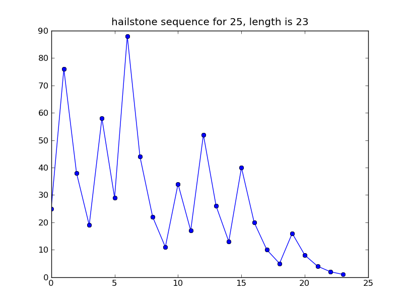
The script will plot the sequence:

$ python collatz.py 25

The Collatz conjecture is is also known as the 3n + 1 conjecture, the Ulam conjecture, Kakutani's problem, the Thwaites conjecture, Hasse's algorithm, or the Syracuse problem; the sequence of numbers involved is referred to as the hailstone sequence or hailstone numbers, or as wondrous numbers.

References

• Numerical Computing with Matlab
• Wikipedia - Collatz conjecture

Integration of a function using quad from scipy

Example of integration of a function using scipy:

from scipy.integrate import quad

f = lambda x: 4-x*x # function to integrate
p = lambda x: (-x*x*x)/3 + 4*x # the primitive of f

# let's try to integrate f in the interval [0 2]
r = quad(f,0,2)   # integration using quad
r_analytic = p(2.0)-p(0.0) # analytic integration

print 'Results'
print r[0]
print r_analytic

Numerical and analytic result compared:

Results
5.33333333333
5.33333333333

Data fitting using fmin

We have seen already how to find the minimum of a function using fmin, in this example we will see how use it to fit a set of data with a curve minimizing an error function:

from pylab import *
from numpy import *
from numpy.random import normal
from scipy.optimize import fmin

# parametric function, x is the independent variable
# and c are the parameters.
# it's a polynomial of degree 2
fp = lambda c, x: c[0]+c[1]*x+c[2]*x*x
real_p = rand(3)

# error function to minimize
e = lambda p, x, y: (abs((fp(p,x)-y))).sum()

# generating data with noise
n = 30
x = linspace(0,1,n)
y = fp(real_p,x) + normal(0,0.05,n)

# fitting the data with fmin
p0 = rand(3) # initial parameter value
p = fmin(e, p0, args=(x,y))

print 'estimater parameters: ', p
print 'real parameters: ', real_p

xx = linspace(0,1,n*3)
plot(x,y,'bo', xx,fp(real_p,xx),'g', xx, fp(p,xx),'r')

show()

The following figure will be showed, in green the original curve used to generate the noisy data, in blue the noisy data and in red the curve found in the minimization process:

The parameters will be printed also:

Optimization terminated successfully.
         Current function value: 0.861885
         Iterations: 77
         Function evaluations: 146
estimater parameters:  [ 0.92504602  0.87328979  0.64051926]
real parameters:  [ 0.86284356  0.95994753  0.67643758]

References

Thursday, June 2, 2011