Neural Networks Regularization made easy with sklearn and matplotlib

Using regularization has many benefits, the most common are reduction of overfitting and solving multicollinearity issues. All of this is covered very well in literature, especially in (Hastie et all). Howerver, wihout touching too many details we can have a very straigthforward interpretation of regularization. Regularization is a way to constrain a model in order to learn less from the data. In this post we will experimentally show what are the effects of regularization on a Neural Network (Multilayer Perceptron) validating this interpretation.

Let's define a goal for our Neural Network. We have a dataset H and we want to build a model able to reconstruct the same data. More formally, we want to build a function f that takes in input H and returns the same values or an approximation close as possible to H. We can say that we want f to minimize the following error

To begin our experiment we build a data matrix H that contains the coordinate of a stylized star:

import numpy as np
import matplotlib.pyplot as plt
%matplotlib inline

x= [np.cos(np.pi/2), 2/5*np.cos(np.pi/2+np.pi/5), np.cos(np.pi/2+2*np.pi/5), 
    2/5*np.cos(np.pi/2+3*np.pi/5), np.cos(np.pi/2+4*np.pi/5), 
    2/5*np.cos(3*np.pi/2), np.cos(np.pi/2+6*np.pi/5), 
    2/5*np.cos(np.pi/2+7*np.pi/5), np.cos(np.pi/2+8*np.pi/5),
    2/5*np.cos(np.pi/2+9*np.pi/5), np.cos(np.pi/2)]

y=[np.sin(np.pi/2), 2/5*np.sin(np.pi/2+np.pi/5), np.sin(np.pi/2+2*np.pi/5),
   2/5*np.sin(np.pi/2+3*np.pi/5), np.sin(np.pi/2+4*np.pi/5),
   2/5*np.sin(3*np.pi/2), np.sin(np.pi/2+6*np.pi/5),
   2/5*np.sin(np.pi/2+7*np.pi/5), np.sin(np.pi/2+8*np.pi/5),
   2/5*np.sin(np.pi/2+9*np.pi/5), np.sin(np.pi/2)]

xp = np.linspace(0, 1, len(x))
np.interp(2.5, xp, x)
x = np.log(np.interp(np.linspace(0, 1, len(x)*10), xp, x)+1)

yp = np.linspace(0, 1, len(y))
np.interp(2.5, yp, y)
y = np.interp(np.linspace(0, 1, len(y)*10), yp, y)
#y[::2] += .1

H = np.array([x, y]).T
plt.plot(H[:,0], H[:,1], '-o')

Now the matrix H contains the x coordinates of our star in the first column and the y coordinates in the second. With the help of sklearn, we can now train a Neural Network and plot the result:

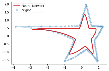
from sklearn.neural_network import MLPRegressor
from sklearn.preprocessing import minmax_scale

H = scale(H)

plt.figure()
f = MLPRegressor(hidden_layer_sizes=(200, 200, 200), alpha=0)
f.fit(H, H)
result = f.predict(H)
plt.plot(result[:,0], result[:,1], 'C3', linewidth=3, label='Neural Network')
plt.plot(H[:,0], H[:,1], 'o', alpha=.3, label='original')
plt.legend()
#plt.xlim([-0.1, 1.1])
#plt.ylim([-0.1, 1.1])
plt.show()

In the snippet above we created a Neural Network with 3 layers of 200 neurons. Then, we trained the model using H as both input and output data. In the chart we compare the original data with the estimation. It's easy to see that there are small differences between the two stars but they are very close.
Here's important to notice that we initialized MLPRegressor using alpha=0. This parameter controls the regularization of the model and the higher its value, the more regularization we apply. To understand how alpha affects the learning of the model we need to add a term to the computation of the error that was just introduced:

where W is a matrix of all the weights in the network. The error not only takes in account the difference between the ouput of the function and the data, but also the size of weights of the connections of the network. Hence, the higher alpha, the less the model is free to learn. If we set alpha to 20 in our experiment we have the following result:

We still achie an approximation of the star but the output of our model is smaller than before and the edges of the star are smoother.
Increasing alpha gradually is a good way to understand the effects of regularization:

from matplotlib.animation import FuncAnimation
from IPython.display import HTML

fig, ax = plt.subplots()
ln, = plt.plot([], [], 'C3', linewidth=3, label='Neural Network')
plt.plot(H[:,0], H[:,1], 'o', alpha=.3, label='original')
plt.legend()

def update(frame):
    f = MLPRegressor(hidden_layer_sizes=(200, 200, 200), alpha=frame)
    f.fit(H, H)
    result = f.predict(H)
    ln.set_data(result[:,0], result[:,1])
    plt.title('alpha = %.2f' % frame)
    return ln,

ani = FuncAnimation(fig, update, frames=np.linspace(0, 40, 100), blit=True)
HTML(ani.to_html5_video())

Here we vary alpha from 0 to 40 and plot the result for each value. We notice here that not only the star gets smaller and smoother as alpha increases but also that the network tends to preserve long lines as much as possible getting away from the edges which account less on error function. Finally we see that the result degenerates into a point when alpha is too high.

Tornado plots with matplotlib

Lately there's a bit of attention about charts where the values of a time series are plotted against the change point by point. This thanks to this rather colorful and cluttered Tornado plot.

In this post we will see how to make one of those charts with our favorite plotting library, matplotlib, and we'll also try to understand how to read them.
Let's start loading the records of the concentration of CO2 in the atmosphere and aggregate the values on month level. After that we can plot straight away the value of the concentration against the change compared to the previous month:

import pandas as pd
import matplotlib.pyplot as plt
%matplotlib inline

data_url = 'ftp://aftp.cmdl.noaa.gov/products/trends/co2/co2_weekly_mlo.txt'
co2_data = pd.read_csv(data_url, sep='\s+', comment='#', na_values=-999.99,
                       names=['year', 'month', 'day', 'decimal', 'ppm', 
                       'days', '1_yr_ago',  '10_yr_ago', 'since_1800'])
co2_data = co2_data.groupby([co2_data.year, co2_data.month]).mean()
idx = co2_data.index.to_flat_index()
co2_data['timestamp'] = [pd.Timestamp(year=y, month=m, day=1) for y, m in idx]
co2_data.set_index('timestamp', inplace=True)
co2_data = co2_data['2018-04-01':]


plt.plot(co2_data.ppm.diff(), co2_data.ppm, '-o')

The result is nicely loopy. This is because we plotted data for 2 years and the time series presents a yearly seasonality. Still, apart from the loop it's quite hard to understand anything without adding few details. Let's print the name of the months and highlight beginning and end of the time series:

from calendar import month_abbr

plt.figure(figsize=(8, 12))
diffs = co2_data.ppm.diff()
plt.plot(diffs, co2_data.ppm, '-o', alpha=.6, zorder=0)
plt.scatter([diffs[1]], [co2_data.ppm[1]],
            c='C0', s=140)
plt.scatter([diffs[-1]], [co2_data.ppm[-1]],
            c='C0', s=140)

for d, v, ts in zip(diffs,
                    co2_data.ppm,
                    co2_data.index):
    plt.text(d, v-.15, '%s\n%d' % (month_abbr[ts.month], ts.year),
             horizontalalignment='left', verticalalignment='top')

plt.xlim([-np.abs(diffs).max()-.1,
          np.abs(diffs).max()+.1])
plt.ylabel('CO2 concentrations (ppm)')
plt.xlabel('change from previous month (ppm)')

The situation is much improved. Now we can see that from June to September (value on the left) the concentrations decrease while from October to May (value on the right) they increase. If we look at the points where the line of zero chance is crossed, we can spot when there's a change of trend. We see that the trend changes from negative to positive from September to October and the opposite from May to June.

Was this easier to observe just have time on the y axis? That's easy to see looking at the chart below.